ALP | Lib. | Nat. | Greens | Teal | Teals+ | |
|---|---|---|---|---|---|---|
MPs | 78 | 50 | 10 | 4 | 6 | 10 |
Ave. % Participation | 82.8 | 62.1 | 59.8 | 84.9 | 90.8 | 89.2 |
Ave. Rice Index | 1 | 0.99 | 1 | 1 | 0.9 | 0.83 |
Ave. Agreement Index | 0.78 | 0.83 | 0.81 | 0.87 | 0.83 | 0.75 |
Note: The total number of MPs for each party may vary from current numbers. Four MPs left the House over the period (Tudge, Robert, Murphy and Morrison, replaced by Caldwell, Doyle, Beylea and Kennedy). Two Coalition MPs (Gee and Broadbent) became independents and so are 'double counted'. The Speaker, Milton Dick, who did not cast a vote, is excluded from the list of ALP MPs. | ||||||
The parliamentary voting behaviour of ‘teal’ independent MPs
Before losing his seat, Dave Sharma (Liberal MP for Wentworth) said of the teals: “If it looks like a political party, if it acts like a political party, if it feels like a political party, I would suggest it is a political party.”
The teal independents are, of course, not formally a party in Australian law1, but their common funder Climate 200 does have a (short) policy platform on which financial support is presumably contingent. They also provide centralised strategic communications, analytics, and training to campaign managers. On the other hand, the label ‘teal’ has been called “lazy journalism—a shorthand to describe what is otherwise a diverse movement of different communities, groups and individuals” (Hendriks and Reid 2023, 293).
The purpose of this post is to revisit the ongoing argument about the ‘party-ness’ of the teals using a criterion other than electoral campaigns and organisation. Using the Parliament of Australia’s Divisions database, I analyse voting patterns in the House of Representatives from June 2022 to present using party cohesion scores, as well as an unfolding technique known as optimal classification (Poole 2000), a form of ideal point analysis.
The results show two things: first, that the teals’ voting coherence was reasonably high, and comparable with the registered parties. There is little to separate them in policy terms, except on votes related to amending the Fair Work Act 2009, which have split the teals several times (in these votes, Victorian teals tended to vote with the government and others with the opposition but not without exception) and occasionally on other divisions including one vote on the Hamas attacks on Israel.
Second, this post reveals the effect that a record 16-strong cross-bench (10 more than the previous high) has had on the structure of parliamentary voting. Voting is now split on two dimensions: a primary government-opposition dimension, and an alternative policy dimension, which splits off minor parties and independents from the two major party groupings. In this two dimensional space, the teals occupy an expected central position between the two major parties on the primary dimension of voting, while occupying a left-of-centre position on the second ‘alternative’ policy dimension.
Recent headlines have shown that the teals’ voting patterns are of interest to the major parties as lines of attack, and this post serves as a fact-based assessment of claims made on this topic. For example, there is Peter Dutton’s recent claim that “Some of the teals – Monique Ryan and Sophie Scamps, they will vote with Labor because they’re Greens, they’re not teals” (Burton 2024). While it’s true that Monique Ryan’s ideal point sits on the left of the teals grouping, Scamps sits closer to the Liberals on the right. In any case, both Ryan and Scamps’s points sit closer to one another than to either the Greens or the Liberals.
Data
The data for this blog came from the Parliament of Australia website, which makes Votes and Proceedings of the House available in machine readable format. The code used to process this data into a format suitable for analysis is available in my teal_ideal github repo. I applied minor modifications to the data in order to account for the departure and arrivals of new MPs mid-term, to record abstentions, and to identify the six independent MPs who were elected for the first time with the help of Climate 200 (Chaney, Daniel, Ryan, Scamps, Spender, and Tink), labelled ‘teals’. I also expanded the definition to also include the four MPs who took Climate 200 funding as part of their reelection campaigns (Steggall, Haines, Wilkie, and Sharkie), labelled ‘teal plus’.
‘Party’ Cohesion
Table 1 gives the number of MPs in each parliamentary grouping, the average division attendance rate among MPs, and two measures of party cohesion, commonly used in the legislative politics literature: the Rice index (1925) and the agreement index (Hix, Noury, and Roland 2005). Beginning with average attendance, cross-bench MPs, including the Greens, attend votes with greater frequency than MPs from major parties. This is explained by two factors. First, MPs from major parties are bound to vote with their party and there are severe sanctions for MPs who ‘cross the floor’. Less severe sanctions exist for abstention, so such MPs who do not support their party may indicate their preference in this way. Second, while attendance is generally required of MPs when major parties divide, only smaller numbers of MPs are required to block motions and bills originating from the cross-bench. This leaves other major party MPs free to use their time in Canberra in different ways. The lowest division attendance rates are typically seen among the government and opposition frontbenches.
Attendance rates provide important context for the two indexes of party cohesion. The Rice index gives the proportion of votes in agreement on a division (equal to 1 when all MPs vote together, and zero when MPs are split evenly) and takes into account only votes for and against a motion, ignoring abstentions. The agreement index extends the rice index to include extensions (equal to one when all MPs vote or abstain together, and zero when MPs are divided evenly across for, against, and abstain).
In the Rice index, all registered political parties score extremely highly. Compared to Westminster, the party discipline is far higher, almost absolute. The only MP of a major party to cross the floor in the parliament so far has been Bridget Archer (Lib.), whose moderate position is widely seen as an important factor in holding her marginal seat. In comparison, teal MPs are more likely to take opposing positions. An average Rice index score of 0.89 compares favourably with scores for Republicans and Democrats in the U.S. House of Representatives, and a little below typical scores for parties in the UK.
Ignoring abstention rates, then, teal independents are approaching the cohesion of fully fledged political party, except that they have no mechanism to enforce parliamentary unity. Applying the agreement index (which takes into account abstention), teal MPs are similarly cohesive to the Australian major parties, suggesting voting behaviour broadly consistent with partisanship.
The teals-plus grouping is less cohesive than the newly-elected teal grouping on both measures. As we will see, this is largely due to the divergent voting patterns of Andrew Wilkie (Ind., Tas.) and Rebekha Sharkie (Centre Alliance, SA). The other two returning teal independents, Zali Steggall (NSW) and Helen Haines (Vic.) were more likely to vote with the core grouping.
Spatial Voting
Next, I take a look at the structure of parliamentary voting at the individual level using the non-parametric optimal classification (OC) model (Poole 2000). OC models (as do other binary unfolding or ideal point models) find an optimal placement for both legislators and divisions in geometric space, usually in one or two dimensions. The algorithm updates until all voting ‘errors’ are minimised; that is, the algorithm will try as far as possible to place division lines between MPs so that the division separates people who voted ‘aye’ from people who voted ‘no’.
The Australian House of Representatives’ standing order 127 makes the current parliament interesting to analyse (and therefore, previous parliaments less interesting): according to House standing orders, full counts of divisions are not made when only four or fewer MPs sit on one side of the Speaker. This long-standing rule is applied as a means to prevent delay tactics by the cross-bench, which numbered six or fewer in every parliament before 2022. In the present parliament, there are more opportunities for the cross-bench to force divisions and move parliamentary voting away from a two-way fight between government and opposition. We see this new dynamic reflected in the results below.
Table 2 gives a summary of two OC models, comparing a one-dimensional solution with the two dimensional solution. As with similar parliamentary legislatures, OC models fit voting behaviour in the House of Representatives with a high degree of accuracy (97.7% correct with one dimension, 99.7% correct with two dimensions). This phenomenon has been termed near ‘perfect spatial voting’ (Rosenthal and Voeten 2004) in that there is rarely any uncertainty in how particular legislators will vote on a given topic, which is a consequence of high party discipline.
1 Dimension | 2 Dimensions | |
|---|---|---|
Number of MPs: | 156 (0 MPs deleted) | 156 (0 MPs deleted) |
Number of Votes: | 387 (3 votes deleted) | 387 (3 votes deleted) |
Predicted Ayes: | 24296 of 24712 (98.3%) predictions correct | 24641 of 24712 (99.7%) predictions correct |
Predicted Noes: | 19425 of 20033 (97%) predictions correct | 19952 of 20033 (99.6%) predictions correct |
Total Proportion Correct: | 0.977 | 0.997 |
Average Proportion Reduction in Error: | 0.934 | 0.99 |
In social science terms, a one dimensional model fits the data well, however, a two dimensional model reduces error even further. Proportional reduction of error is a fit statistic which calculates the improvement the model makes over a ‘null-model’, in which everyone is predicted to vote with the majority, and is the ratio of the difference between the number of votes in the minority and the number of classification errors, over the total number of votes in the minority. The average proportional reduction in error (APRE) is simply the aggregated mean of PRE statistics over all divisions. The APRE improves markedly from 0.93 to 0.99 in two dimensions, suggesting that while the first dimension is by far the dominant predictor, including a second dimension produces the better model fit.
Now to interpret the model results.2 Figure 1 shows the estimated positions of MPs and the dividing lines for each vote. This plot is available to examine interactively, using the mouse to hover over and provide contextual information. Using the hover tool, it is easy to see (by hovering the mouse over the edge of the perimeter circle) who introduces each division, their party, the turnout, and the topic. It is also possible to see the positions of individual MPs. To aid the reader, I have traced the ‘convex hulls’ of party groupings to show their spatial limits: red for the ALP, blue for the Coalition, green for the Greens, teal with solid line for the teals, and teal with dashed lines for the teals-plus.
The first dimension represents a government-opposition dynamic. Both Labor and the Liberal-National Coalition sit at the extremes in strategic opposition (Dewan and Spirling 2011). Tight government agenda control over motions ensures that cross-bench MPs are aligned in between, as they vote for or against the government. The second dimension accounts for a cleavage between the majority of cross-bench MPs (with the notable exception of Bob Katter) and the major parties, which I term ‘alternative policy’.
A look at who introduces divisions which separate on the alternative dimension (horizontal lines) reveals that they are disproportionately introduced by cross-bench MPs. Further, divisions which discriminate on this dimension are also strongly associated with low turnout. This is likely because major parties do not need to whip many MPs to vote on motions which do not split the major parties. Figure 2 shows the relationship between the angle of the cutting line (where horizontal lines equal 0 and vertical lines equal 90) and turnout on divisions. The lower the cutting angle of a division, the more associated with the alternative policy dimension it becomes. The scatter plot describes a correlation coefficient between turnout and cutting angle of 0.77, which suggests that motions proposed by cross-benchers do not require full participation of government or opposition to block.
Finally, a qualitative glance at the topics of divisions in this dimension suggests that alternative policy positions, often on climate change are being debated and voted on more frequently with the current cross-bench. Some examples are:
So, are the teals a party?
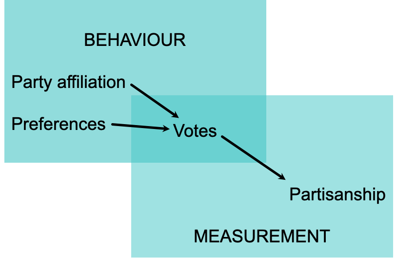
Nearly a quarter of a century ago, Keith Krehbiel (2000) encapsulated the problem of measuring partisanship from votes: by the time we observe voting behaviour, it is too late to separate the twin causes of legislative voting (an MP’s partisan affiliation and their personal preference). The teals certainly vote with the sort of cohesion that qualifies for a party in many parliamentary democracies, but maybe not to the iron discipline required of Australian parties. Perhaps if they were a formal party, their vote attendance (now the highest of the parliamentary groups) would go down to accommodate the occasional strategic abstention. It’s also true that it makes strategic sense for the teals to vote with some cohesion — with a minimum threshold to recording divisions currently set at 4 members, teals will have to coordinate to ensure they have their voices heard.
If we can consider the teals a quasi-party based on voting record, then, who exactly are they? Referring back to the spatial analysis, it makes sense to categorise the 2022 teals, alongside Helen Haines and Zali Steggall as a core grouping. Other established independents Andrew Wilkie (formerly Green) and Rebekha Sharkie who also took Climate 200 money for re-election diverge significantly from the others, and should be considered functionally independent. Of course, it does not (yet) make any sense to call a particular MP a ‘true’ teal or teal-in-name-only (as Dutton might refer to Monique Ryan or Sophie Scamps) based on voting record.
References
Armstrong, David A., Ryan Bakker, Royce Carroll, Christopher Hare, Keith T. Poole, and Howard Rosenthal. 2020. Analyzing Spatial Models of Choice and Judgment. 2nd ed. New York: Chapman; Hall/CRC. https://doi.org/10.1201/9781315197609.
Australian Electoral Commission. 2023. “Guide for Registering a Party.”
Burton, Tom. 2024. “Dutton Won’t Release 2030 Emission Targets till After Election.” https://www.afr.com/politics/federal/more-bird-flu-infection-outbreaks-predicted-20240610-p5jkq7.
Dewan, Torun, and Arthur Spirling. 2011. “Strategic Opposition and Government Cohesion in Westminster Democracies.” American Political Science Review 105 (2): 337358.
Hendriks, Carolyn M, and Richard Reid. 2023. “The Rise and Impact of Australia’s Movement for Community Independents.” In, edited by Marian Sawer, Anika Gauja, and Jill Sheppard. ANU E Press.
Hix, Simon, Abdul Noury, and Gérard Roland. 2005. “Power to the Parties: Cohesion and Competition in the European Parliament, 19792001.” British Journal of Political Science 35 (02): 209234.
Krehbiel, Keith. 2000. “Party Discipline and Measures of Partisanship.” American Journal of Political Science 44 (2): 206221.
Poole, Keith T. 2000. “Nonparametric Unfolding of Binary Choice Data.” Political Analysis 8 (3): 211–37. https://doi.org/10.1093/oxfordjournals.pan.a029814.
Rice, Stuart A. 1925. “The Behavior of Legislative Groups: A Method of Measurement.” Political Science Quarterly 40 (1): 6072.
Rosenthal, Howard, and Erik Voeten. 2004. “Analyzing Roll Calls with Perfect Spatial Voting: France 1946-1958.” American Journal of Political Science 48 (3): 620–32. https://doi.org/10.2307/1519920.
Slapin, Jonathan B., Justin H. Kirkland, Joseph A. Lazzaro, Patrick A. Leslie, and Tom O’grady. 2018. “Ideology, Grandstanding, and Strategic Party Disloyalty in the British Parliament.” American Political Science Review 112 (1): 15–30. https://doi.org/10.1017/S0003055417000375.
Spirling, Arthur, and Iain McLean. 2007. “UK OC OK? Interpreting Optimal Classification Scores for the UK House of Commons.” Political Analysis 15 (1): 85–96.
Footnotes
The legal definition includes important criteria, but ultimately allows any group with a constitution, $500 and 1500 members to receive registration (Australian Electoral Commission 2023).↩︎
For nerds: I need to address two common objections to the use of ideal point models in parliamentary democracy. First, parametric models assume independent and identical distribution (i.i.d.) of error terms when estimating the ideal points of individuals. This assumption is potentially problematic in all analysis of roll call data, but it is particularly troublesome in settings where some parliamentary groupings are known to be more disciplined than others, as in the present case. The OC model is non-parametric, and so relaxes assumptions about the form and consistency of the error term, as argued in Rosenthal and Voeten (2004) and Armstrong et al. (2020).
Second, interpretations of rollcall analysis in parliamentary settings sometimes lack face validity when estimating the ideological positions of legislators because government-opposition dynamics usually override individual ‘sincere’ ideology as a predictor of vote choice. Legislators who cross the floor appear as moderates (Spirling and McLean 2007), though they are often extremists within their parties who rebel strategically to signal their opposition to the centrism of the party leadership (Slapin et al. 2018). For this reason, I do not interpret the results for the major parties in terms of individual ideological positions on a left-right spectrum. In any case, the cohesion scores show that the differences in position among parties are driven almost entirely by abstentions. It’s not possible to know whether these abstentions are strategic or not.↩︎